Our project goal was to test if the distribution of player salaries correlates to a team’s success in the NBA, NFL, and MLB over the last 20 years. We hypothesized that salary inequality (some players making more money than others on the team) will be positively correlated with team success in the NBA, but negatively associated with team success in MLB and the NFL.
We chose to perform statistical tests because our goal is to explore the relationship between two variables: salary distribution and win rate. If our goal was to create the most accurate predictor of win rate, we would have turned to machine learning and added several more features to increase the model’s predictive power.
Because we performed statistical tests, our quantitative measures of success were the resulting p-values. Of course, a failure to reject a null hypothesis due to a high p-value is not a “failure” in the sense of a bad result. A failure to reject a null hypothesis is a successful outcome in its own right.
Before we performed statistical tests, we first needed to preprocess the data. For each team, the win rate and salaries of the n (15, 25, 50 for NBA, MLB, NFL, respectively) most highly paid players were retrieved. The value of n differs based on the sport because football teams, for example, tend to have many more players on their roster than in basketball. Salaries were then normalized as a percentage of total salary expenditure on a per team basis. These normalized salary distributions were then binned by win rate, with one group having a win rate greater than the median, and the other less than the median, excluding those equal to the median. Note that, as might be expcted, the median winrate was ~0.5 in all three sports. Thus, we were left with two groups of salary distributions - one for high win rate and one for low win rate.
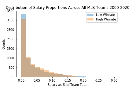
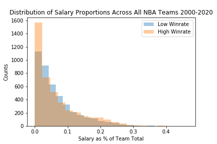
First, we wanted to explore the data by visualizing how the salary distributions for high win-rate and low win-rate teams differed. Figures 1-3 show these distributions for all three sports. It should be noted that the axis scales differ across sports as we have different amounts of team data and player data for each sport. For example, we were only able to collect NFL data for 2000-2010, but because NFL teams have more players than NBA teams, the amount of player salaries we observed is about the same. For a similar reason, the x-axis scale differs as well. If a team has more players (e.g. NFL teams), each player will receive a smaller percentage of the total salary.
From a first glance, there appear to be slight differences in the NBA and MLB distributions for high v. low win-rate teams, but not in the NFL. Interestingly, it appears that high winrate teams in the NBA tend to have more low-paid players as well as more high-paid players (i.e. top-heavy) than low winrate teams, while in the MLB this trend is reversed. This is a first indication that salary distribution might be correlated with winrate differently across sports. In order to test our visual intuition on the differences between the distribution, we employed a two-sample Kolmogorov-Smirnov test. The Kolmogorv-Smirnov test is a two-sample non-parametric statistical test that quantifies the difference between two empirical distributions. In our case, the two empirical distributions are the concatenated salary distributions of high win-rate and low win-rate teams. Table 1 shows the results of this test for all three sports. We see that the p-values are less than 0.05 for NBA and MLB but not for NFL, matching our intuition.
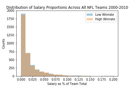
| Sport | P-value |
|---|---|
| NBA | 8.211e-17 |
| MLB | 8.0812e-13 |
| NFL | 0.156 |
The results of the Kolmogorov-Smirnov tests mainly serve as an indication that salary inequality could be correlated with win-rate. It only shows that the salary distributions between low and high win-rate teams are different- it makes no statement or assumption about how the distributions are shaped. To test our actual hypothesis - whether salary inequality is associated with win rate - we must incorporate a quantified notion of salary inequality in our test.
The Gini coefficient is a well-known measure of statistical dispersion that is commonly used to measure wealth inequality. A higher Gini coefficient implies greater inequality. In the context of salary distributions on a team, a higher Gini coefficient suggests that a team is “top-heavy”, meaning that a few players are paid disproportionately more than the rest of the team.
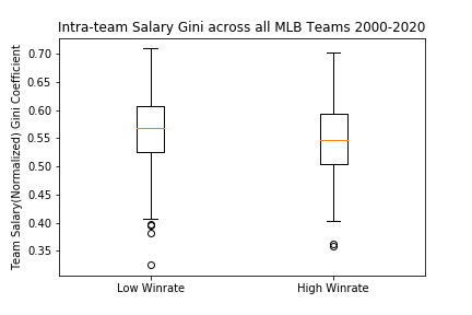
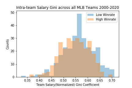
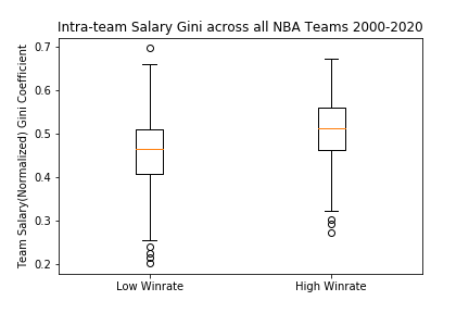
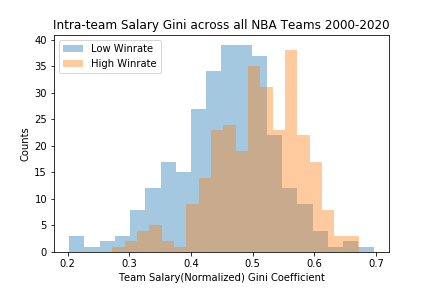
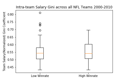
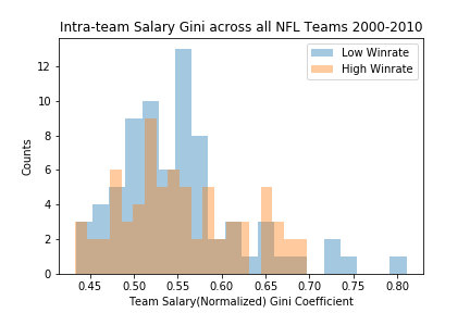
Figures 4-6 show the distributions of Gini in each sport. For each sport, we include a box plot and a histogram. The box plot displays the mean and outliers of Gini, while the histogram displays the overall shape of the distribution for high and low win rates. We observe that Gini is higher (i.e. more “top-heavy”) for high win-rate teams in the NBA, higher for low win-rate teams in the MLB, and roughly the same in the NFL. We also include Table 2 with results of this test for all three sports.
| Sport | P-value |
|---|---|
| NBA | 1.903e-15 |
| MLB | 0.0005 |
| NFL | 0.918 |
After visualizing the Gini distributions, we conducted two statistical tests to investigate our hypothesis: a two-sample T-test and multiple-linear regression.
Two Sample T-Test
The two-sample T-test tested whether Gini is significantly different between high and low win-rate teams. In this sense, we are indirectly testing whether Gini is related to win-rate. Table 2 shows the results for these tests in each sport. We see that there is a significant difference (p < 0.05) in the NBA and MLB, but not the NFL. Therefore, we reject the null hypothesis that there is no difference in Gini between low and high win-rate teams in the NBA and MLB. Interestingly, the results are significant in opposite directions: higher win-rate teams have significantly higher Gini coefficients in the NBA, whereas they are significantly lower in the MLB.
Multiple-Linear Regression
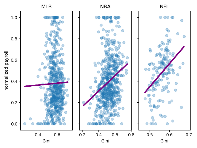
We need to run a multiple regression because payroll and Gini are correlated, so in a simple linear regression with win rate as the dependent varaible and Gini as the independent variable it would be impossible to tell if the observed relationship has anything to do with Gini or if payroll is a lurking variable influencing the result. Figure 7 shows that there is a clear correlation between Gini and Payroll.
The independent variables we used for multiple-linear regression are Gini and total payroll, and the dependent variable is win-rate. We are really only interested in the relationship between Gini and win rate, but since payroll clearly influences both Gini and win rate, we need to determine that the previously observed relationship between Gini and win rate is not mediated by payroll. Table 3 shows the results of these tests.
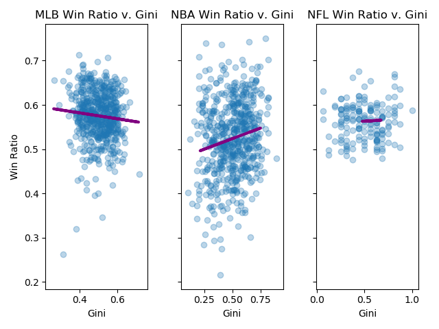
The R^2 values for all three sports are low, especially in the NFL. We interpret this to mean that Gini and payroll accounts for only a small portion of the variance in win-rate. There are likely many other factors (e.g. team chemistry, facilities, resources) that account for the remainder of the variation. Nevertheless, the p-values for the Gini coefficient suggest that there are significant results for the NBA and MLB but not for NFL. Therefore, we reject the null hypothesis that there is no correlation between Gini and win-rate in the NBA and MLB. In particular, there is a significant positive correlation between Gini and win-rate in the NBA, and a significant negative correlation between the two in the MLB. Although we cannot display the graphs for multiple-linear regression, we generated graphs for simple linear-regression between Gini and win-rate for all sports that showcase the same trend. They are shown in Figure 8.
| Sport | Regression coefficient for Gini | P-value for Gini | R^2 |
|---|---|---|---|
| NBA | 0.1665 | 0.021 | 0.114 |
| MLB | -0.1173 | 0.016 | 0.170 |
| NFL | -0.1473 | 0.719 | 0.050 |
The results of our three tests agree with each other. The Kolmogorov-Smirnov test showed that there were significant differences in salary distributions between high and low win-rate teams in the NBA and MLB. The two sample T-test expanded upon this result by showing that there was a significant difference in Gini, or salary inequality, between the two groups. In particular, high win-rate teams in the NBA had a higher Gini, whereas low win-rate teams in the MLB had a higher Gini. Multi-linear regression verified this result by indicating a significant positive correlation between Gini and win-rate in the NBA and a significant negative correlation between Gini and win-rate in the MLB.
All three results suggested that salary distribution had an insignificant effect on win-rate in the NFL. We hypothesize that our lack of NFL data made it difficult to evaluate our model regarding that sport. Given more time, we may have overcome this challenge by compiling more NFL data from other sources. However, it may also be the case that this trend truly doesn’t exist in the NFL, or at least to a lesser extent due to the abundance of players on football teams. As the total salary is split among more than twice as many players as in basketball or baseball, it becomes less feasible for individual player salaries to signficantly deviate from a uniform expectation.
Perhaps MLB Front Offices would be well-advised to spend evenly on players while NBA Front Offices would be well-advised to spend big on a superstar or two at the expense of the rest of the roster.